regression: Simple Linear Regression (by Hand)
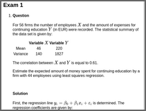
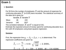
regressionFor 56 firms the number of employees \(X\) and the amount of expenses for continuing education \(Y\) (in EUR) were recorded. The statistical summary of the data set is given by:
| Variable \(X\) | Variable \(Y\) | |
|---|---|---|
| Mean | 46 | 220 |
| Variance | 140 | 1827 |
The correlation between \(X\) and \(Y\) is equal to 0.61.
Estimate the expected amount of money spent for continuing education by a firm with 44 employees using least squares regression.
First, the regression line \(y_i = \beta_0 + \beta_1 x_i + \varepsilon_i\) is determined. The regression coefficients are given by: \[\begin{eqnarray*} && \hat \beta_1 = r \cdot \frac{s_y}{s_x} = 0.61 \cdot \sqrt{\frac{1827}{140}} = 2.20361, \\ && \hat \beta_0 = \bar y - \hat \beta_1 \cdot \bar x = 220 - 2.20361 \cdot 46 = 118.63386. \end{eqnarray*}\]
The estimated amount of money spent by a firm with 44 employees is then given by: \[\begin{eqnarray*} \hat y = 118.63386 + 2.20361 \cdot 44 = 215.593. \end{eqnarray*}\]
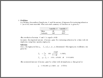
For 46 firms the number of employees \(X\) and the amount of expenses for continuing education \(Y\) (in EUR) were recorded. The statistical summary of the data set is given by:
| Variable \(X\) | Variable \(Y\) | |
|---|---|---|
| Mean | 44 | 236 |
| Variance | 78 | 1644 |
The correlation between \(X\) and \(Y\) is equal to 0.76.
Estimate the expected amount of money spent for continuing education by a firm with 40 employees using least squares regression.
First, the regression line \(y_i = \beta_0 + \beta_1 x_i + \varepsilon_i\) is determined. The regression coefficients are given by: \[\begin{eqnarray*} && \hat \beta_1 = r \cdot \frac{s_y}{s_x} = 0.76 \cdot \sqrt{\frac{1644}{78}} = 3.48913, \\ && \hat \beta_0 = \bar y - \hat \beta_1 \cdot \bar x = 236 - 3.48913 \cdot 44 = 82.47826. \end{eqnarray*}\]
The estimated amount of money spent by a firm with 40 employees is then given by: \[\begin{eqnarray*} \hat y = 82.47826 + 3.48913 \cdot 40 = 222.043. \end{eqnarray*}\]
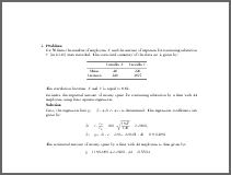
For 65 firms the number of employees \(X\) and the amount of expenses for continuing education \(Y\) (in EUR) were recorded. The statistical summary of the data set is given by:
| Variable \(X\) | Variable \(Y\) | |
|---|---|---|
| Mean | 44 | 259 |
| Variance | 93 | 2529 |
The correlation between \(X\) and \(Y\) is equal to 0.83.
Estimate the expected amount of money spent for continuing education by a firm with 38 employees using least squares regression.
First, the regression line \(y_i = \beta_0 + \beta_1 x_i + \varepsilon_i\) is determined. The regression coefficients are given by: \[\begin{eqnarray*} && \hat \beta_1 = r \cdot \frac{s_y}{s_x} = 0.83 \cdot \sqrt{\frac{2529}{93}} = 4.32824, \\ && \hat \beta_0 = \bar y - \hat \beta_1 \cdot \bar x = 259 - 4.32824 \cdot 44 = 68.55757. \end{eqnarray*}\]
The estimated amount of money spent by a firm with 38 employees is then given by: \[\begin{eqnarray*} \hat y = 68.55757 + 4.32824 \cdot 38 = 233.031. \end{eqnarray*}\]
(Note that the HTML output contains mathematical equations in MathML, rendered by MathJax using ‘mathjax = TRUE’. Instead it is also possible to use ‘converter = “pandoc-mathjax”’ so that LaTeX equations are rendered by MathJax directly.)
Demo code:
library("exams")

set.seed(403)
exams2html("regression.Rmd", mathjax = TRUE)
set.seed(403)
exams2pdf("regression.Rmd")

set.seed(403)
exams2html("regression.Rnw", mathjax = TRUE)
set.seed(403)
exams2pdf("regression.Rnw")


